![[DBPP]](3_9 Case Study Shortest-Path Algorithms.files/asm_color_tiny.gif)


![[Search]](3_9 Case Study Shortest-Path Algorithms.files/search_motif.gif)
We conclude this chapter by using performance models to compare four different parallel algorithms for the all-pairs shortest-path problem. This is an important problem in graph theory and has applications in communications, transportation, and electronics problems. It is interesting because analysis shows that three of the four algorithms can be optimal in different circumstances, depending on tradeoffs between computation and communication costs.
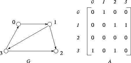
Figure 3.23: A simple directed graph, G, and its
adjacency matrix, A.
The all-pairs shortest-path problem involves finding the shortest path
between all pairs of vertices in a graph. A graph G=(V,E) comprises a
set V of N vertices,  , and a set
E
, and a set
E  V of
edges connecting vertices in V . In a directed graph, each edge also
has a direction, so edges
V of
edges connecting vertices in V . In a directed graph, each edge also
has a direction, so edges  and
and  ,
,  , are distinct. A
graph can be represented as an adjacency matrix A in which each element
(i,j) represents the edge between element i and j .
, are distinct. A
graph can be represented as an adjacency matrix A in which each element
(i,j) represents the edge between element i and j .
 if there is an
edge
if there is an
edge  ; otherwise,
  =0
(Figure 3.23).
=0
(Figure 3.23).
A path from vertex  to vertex
  is a sequence of
edges
is a sequence of
edges  ,
,  , ...,
  from E
in which no vertex appears more than once. For example,
from E
in which no vertex appears more than once. For example,  ,
,  is a path from
vertex 1 to vertex 0 in Figure 3.23. The
shortest path between two vertices
is a path from
vertex 1 to vertex 0 in Figure 3.23. The
shortest path between two vertices  and
and  in a graph is
the path that has the fewest edges. The
single-source shortest-path problem requires that we find the shortest
path from a single vertex to all other vertices in a graph. The all-pairs
shortest-path problem requires that we find the shortest path between all
pairs of vertices in a graph. We consider the latter problem and present four
different parallel algorithms, two based on a sequential shortest-path algorithm
due to Floyd and two based on a sequential algorithm due to Dijkstra. All four
algorithms take as input an N
in a graph is
the path that has the fewest edges. The
single-source shortest-path problem requires that we find the shortest
path from a single vertex to all other vertices in a graph. The all-pairs
shortest-path problem requires that we find the shortest path between all
pairs of vertices in a graph. We consider the latter problem and present four
different parallel algorithms, two based on a sequential shortest-path algorithm
due to Floyd and two based on a sequential algorithm due to Dijkstra. All four
algorithms take as input an N  N
adjacency matrix A and compute an N
N
adjacency matrix A and compute an N  N matrix S , with
  the length of
the shortest path from
the length of
the shortest path from  to
to  , or a
distinguished value (
, or a
distinguished value ( ) if there is no
path.
) if there is no
path.
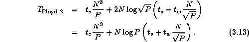
Floyd's all-pairs shortest-path algorithm is given as
Algorithm 3.1. It
derives the matrix S in N steps,
constructing at each step k an intermediate matrix I(k)
containing the best-known shortest distance between each pair of nodes.
Initially, each  is set to the
length of the edge
is set to the
length of the edge  , if the edge
exists, and to
, if the edge
exists, and to  otherwise. The
k th step of the algorithm considers each
otherwise. The
k th step of the algorithm considers each  in turn
and determines whether the best-known path from
in turn
and determines whether the best-known path from  to
to  is longer than
the combined lengths of the best-known paths from
is longer than
the combined lengths of the best-known paths from  to
to  and from
  to
to  . If so, the
entry
. If so, the
entry  is updated to
reflect the shorter path (Figure 3.24). This
comparison operation is performed a total of
is updated to
reflect the shorter path (Figure 3.24). This
comparison operation is performed a total of  times; hence, we
can approximate the sequential cost of this algorithm as
times; hence, we
can approximate the sequential cost of this algorithm as  ,
where
,
where  is the cost of a
single comparison operation.
is the cost of a
single comparison operation.
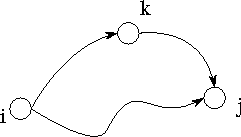
Figure 3.24: The fundamental operation in Floyd's
sequential shortest-path algorithm: Determine whether a path going from  to
to  via
via  is shorter than
the best-known path from
is shorter than
the best-known path from  to
to  .
.
The first parallel Floyd algorithm is based on a one-dimensional, rowwise domain decomposition of the intermediate matrix I and the output matrix S . Notice that this means the algorithm can use at most N processors. Each task has one or more adjacent rows of I and is responsible for performing computation on those rows. That is, it executes the following logic.
for i
= local_i_start to local_i_end
for j = 0
to N-1
endfor
endfor
endfor
for k = 0
to N-1
 (k+1) = min(
 (k),
(k),  (k)+
(k)+ (k))
(k))
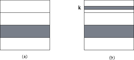
Figure 3.25: Parallel version of Floyd's algorithm
based on a one-dimensional decomposition of the I matrix. In (a), the
data allocated to a single task are shaded: a contiguous block of rows. In (b),
the data required by this task in the k th step of the algorithm are
shaded: its own block and the k th row.
In the k th step, each task requires, in addition to its local data,
the values  ,
,  , ...,
  , that is, the
k th row of I (Figure 3.25).
Hence, we specify that the task with this row broadcast it to all other tasks.
This communication can be performed by using a tree structure in
, that is, the
k th row of I (Figure 3.25).
Hence, we specify that the task with this row broadcast it to all other tasks.
This communication can be performed by using a tree structure in  steps. Because
there are N such broadcasts and each message has size N , the
cost is
steps. Because
there are N such broadcasts and each message has size N , the
cost is
Notice that each task must serve as the ``root'' for at least one broadcast
(assuming  ). Rather than
defining P binary tree structures, it suffices to connect the
P tasks using a hypercube structure (Chapter 11),
which has the useful property of allowing any node to broadcast to all other
nodes in
). Rather than
defining P binary tree structures, it suffices to connect the
P tasks using a hypercube structure (Chapter 11),
which has the useful property of allowing any node to broadcast to all other
nodes in  steps.
An alternative parallel version of Floyd's algorithm uses a two-dimensional
decomposition of the various matrices. This version allows the use of up to  processors and
requires that each task execute the following logic.
processors and
requires that each task execute the following logic.
for i
= local_i_start to local_i_end
for j
= local_j_start to local_j_end
endfor
endfor
endfor
for k = 0
to N-1
 (k+1) = min(
 (k),
(k),  (k)+
(k)+ (k))
(k))
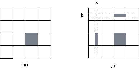
Figure 3.26: Parallel version of Floyd's algorithm
based on a two-dimensional decomposition of the I matrix. In (a), the
data allocated to a single task are shaded: a contiguous submatrix. In (b), the
data required by this task in the k th step of the algorithm are
shaded: its own block, and part of the k th row and column.
In each step, each task requires, in addition to its local data,  values from two
tasks located in the same row and column of the 2-D task array (Figure 3.26).
Hence, communication requirements at the k th step can be structured as
two broadcast operations: from the task in each row that possesses part of
column k to all other tasks in that row, and from the task in each
column that possesses part of row k to all other tasks in that column.
values from two
tasks located in the same row and column of the 2-D task array (Figure 3.26).
Hence, communication requirements at the k th step can be structured as
two broadcast operations: from the task in each row that possesses part of
column k to all other tasks in that row, and from the task in each
column that possesses part of row k to all other tasks in that column.
In each of N steps,  values must be
broadcast to the
values must be
broadcast to the  tasks in each
row and column, and the total cost is
tasks in each
row and column, and the total cost is
Notice that each task must serve as the ``root'' node for at least one broadcast to each task in the same row and column of the 2-D task array. These communication requirements can be satisfied by connecting tasks in the same row or column in a hypercube structure.
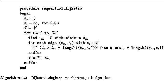
Dijkstra's single-source shortest-path
algorithm computes all shortest paths from a single
vertex,  . It can also be
used for the all-pairs shortest-path problem, by the
simple expedient of applying it N times---once to each vertex
. It can also be
used for the all-pairs shortest-path problem, by the
simple expedient of applying it N times---once to each vertex  , ...,
  .
.
Dijkstra's sequential single-source algorithm is given as Algorithm 3.2. It
maintains as T the set of vertices for which shortest paths have not
been found, and as  the shortest
known path from
the shortest
known path from  to vertex
  . Initially,
T=V and all
. Initially,
T=V and all  . At each step of
the algorithm, the vertex
. At each step of
the algorithm, the vertex  in T
with the smallest d value is removed from T . Each neighbor of
in T
with the smallest d value is removed from T . Each neighbor of
 in T is
examined to see whether a path through
in T is
examined to see whether a path through  would be shorter
than the currently best-known path (Figure 3.27).
would be shorter
than the currently best-known path (Figure 3.27).
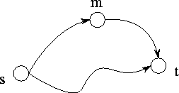
Figure 3.27: The comparison operation performed in
Dijkstra's single-source shortest-path algorithm. The best-known path from the
source vertex  to vertex
  is compared with
the path that leads from
is compared with
the path that leads from  to
to  and then to
  .
.
An all-pairs algorithm executes Algorithm 3.2
N times, once for each vertex. This involves  comparisons and takes time
  F ,
where
F ,
where  is the cost of a
single comparison in Floyd's algorithm and F is a constant. Empirical
studies show that F
is the cost of a
single comparison in Floyd's algorithm and F is a constant. Empirical
studies show that F  1.6; that is,
Dijkstra's algorithm is slightly more expensive than Floyd's algorithm.
1.6; that is,
Dijkstra's algorithm is slightly more expensive than Floyd's algorithm.
The first parallel Dijkstra algorithm replicates the graph in each of P tasks. Each task executes the sequential algorithm for N/P vertices. This algorithm requires no communication but can utilize at most N processors. Because the sequential Dijkstra algorithm is F times slower than the sequential Floyd algorithm, the parallel algorithm's execution time is

The second parallel Dijkstra algorithm allows for the case when
P>N . We define N sets of P/N tasks. Each set of
tasks is given the entire graph and is responsible for computing shortest paths
for a single vertex (Figure 3.28).
Within each set of tasks, the vertices of the graph are partitioned. Hence, the
operation Find  with minimum

requires first a local computation to find the local vertex with minimum
d and second a reduction involving all P/N tasks in the same
set in order to determine the globally minimum  . The reduction
can be achieved by using the butterfly communication structure of Section 2.4.1, in
. The reduction
can be achieved by using the butterfly communication structure of Section 2.4.1, in
 steps. Hence, as
the reduction is performed N times and involves two values, the total
cost of this algorithm is
steps. Hence, as
the reduction is performed N times and involves two values, the total
cost of this algorithm is

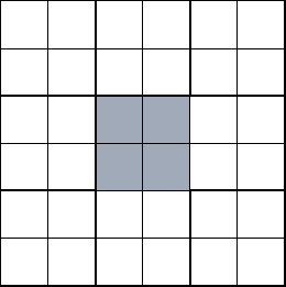
Figure 3.28: The second parallel Dijkstra algorithm
allocates P/N tasks to each of N instantiations of Dijkstra's
single-source shortest-path algorithm. In this figure, N=9 and
P=36 , and one set of P/N=4 tasks is shaded.
Table 3.7
summarizes the performance models developed for the four
all-pairs shortest-path algorithms. Clearly, Floyd 2 will always be more
efficient that Floyd 1. Both algorithms have the same computation costs and send
the same number of messages, but Floyd 2 communicates considerably less data. On
the other hand, Floyd 1 is easier to implement. Algorithms Dijkstra 1 and 2 will
be more efficient than Floyd 2 in certain circumstances. For example, Dijkstra 1
is more efficient than Floyd 2 if P  N and
N and

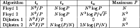
Table 3.7: Performance of four parallel shortest-path
algorithms.
In addition to these factors, we must consider the fact that algorithms Dijkstra 1 and Dijkstra 2 replicate the graph P and P/N times, respectively. This replication may compromise the scalability of these algorithms. Also, the cost of replicating an originally distributed graph must be considered if (as is likely) the shortest-path algorithm forms part of a larger program in which the graph is represented as a distributed data structure.
Clearly, the choice of shortest-path algorithm for a particular problem will involve complex tradeoffs between flexibility, scalability, performance, and implementation complexity. The performance models developed in this case study provide a basis for evaluating these tradeoffs.
© Copyright 1995 by Ian Foster