![[DBPP]](2_3 Communication_files/asm_color_tiny.gif)


![[Search]](2_3 Communication_files/search_motif.gif)
The tasks generated by a partition are intended to execute concurrently but cannot, in general, execute independently. The computation to be performed in one task will typically require data associated with another task. Data must then be transferred between tasks so as to allow computation to proceed. This information flow is specified in the communication phase of a design.
Recall from Chapter 1 that in our programming model, we conceptualize a need for communication between two tasks as a channel linking the tasks, on which one task can send messages and from which the other can receive. Hence, the communication associated with an algorithm can be specified in two phases. First, we define a channel structure that links, either directly or indirectly, tasks that require data (consumers) with tasks that possess those data (producers). Second, we specify the messages that are to be sent and received on these channels. Depending on our eventual implementation technology, we may not actually create these channels when coding the algorithm. For example, in a data-parallel language, we simply specify data-parallel operations and data distributions. Nevertheless, thinking in terms of tasks and channels helps us to think quantitatively about locality issues and communication costs.
The definition of a channel involves an intellectual cost and the sending of a message involves a physical cost. Hence, we avoid introducing unnecessary channels and communication operations. In addition, we seek to optimize performance by distributing communication operations over many tasks and by organizing communication operations in a way that permits concurrent execution.
In domain decomposition problems, communication requirements can be difficult to determine. Recall that this strategy produces tasks by first partitioning data structures into disjoint subsets and then associating with each datum those operations that operate solely on that datum. This part of the design is usually simple. However, some operations that require data from several tasks usually remain. Communication is then required to manage the data transfer necessary for these tasks to proceed. Organizing this communication in an efficient manner can be challenging. Even simple decompositions can have complex communication structures.
In contrast, communication requirements in parallel algorithms obtained by functional decomposition are often straightforward: they correspond to the data flow between tasks. For example, in a climate model broken down by functional decomposition into atmosphere model, ocean model, and so on, the communication requirements will correspond to the interfaces between the component submodels: the atmosphere model will produce values that are used by the ocean model, and so on (Figure 2.3).
In the following discussion, we use a variety of examples to show how communication requirements are identified and how channel structures and communication operations are introduced to satisfy these requirements. For clarity in exposition, we categorize communication patterns along four loosely orthogonal axes: local/global, structured/unstructured, static/dynamic, and synchronous/asynchronous.
A local communication structure is obtained when an operation requires data from a small number of other tasks. It is then straightforward to define channels that link the task responsible for performing the operation (the consumer) with the tasks holding the required data (the producers) and to introduce appropriate send and receive operations in the producer and consumer tasks, respectively.
For illustrative purposes, we consider the
communication requirements associated with a simple numerical computation,
namely a Jacobi finite difference method. In this class of numerical method, a
multidimensional grid is repeatedly updated by replacing the value at each point
with some function of the values at a small, fixed number of neighboring points.
The set of values required to update a single grid point
is called that grid point's stencil. For example, the following
expression uses a five-point stencil to update each element  of a two-dimensional
grid X :
of a two-dimensional
grid X :
This update is applied repeatedly to compute a sequence of values  ,
,  , and so
on. The notation
, and so
on. The notation  denotes the value of grid point
  at step
t .
at step
t .
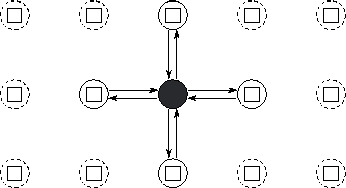
Figure 2.4:
Task and channel structure for a two-dimensional finite difference
computation with five-point update stencil. In this simple fine-grained
formulation, each task encapsulates a single element of a two-dimensional grid
and must both send its value to four neighbors and receive values from four
neighbors. Only the channels used by the shaded task are shown.
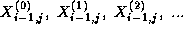
Let us assume that a partition has used domain decomposition techniques to
create a distinct task for each point in the two-dimensional grid. Hence, a task
allocated the grid point  must compute the sequence
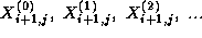
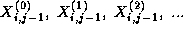
This computation requires in turn the four corresponding sequences
which are produced by the four tasks handling grid points
 ,
,  ,
,  , and
, and  , that is,
by its four neighbors in the grid. For these values to be communicated, we
define channels linking each task that requires a value with the task that
generates that value. This yields the channel structure illustrated in Figure 2.4. Each
task then executes the following logic:
, that is,
by its four neighbors in the grid. For these values to be communicated, we
define channels linking each task that requires a value with the task that
generates that value. This yields the channel structure illustrated in Figure 2.4. Each
task then executes the following logic:
for t=0 to T-1send
to each neighbor
receive
,
,
,
from neighbors
compute
using Equation 2.1
endfor
We observed earlier that the best sequential and parallel solutions to a
problem may use different techniques. This situation arises in finite difference
problems. In sequential computing, Gauss-Seidel update
strategies are often preferred over Jacobi strategies because they allow
solutions of comparable accuracy to be obtained using fewer iterations. In a
Gauss-Seidel scheme, elements are updated in a particular order so that the
computation of each element can use the most up-to-date value of other elements.
For example, the Jacobi update of Equation 2.1 may be
reformulated as follows (notice the use of values  and
and  ):
):
While Jacobi schemes are trivial to parallelize (all grid points can be
updated concurrently), this is not the case for all Gauss-Seidel schemes. For example, the update scheme of Equation 2.2 allows
only an average of around N/2 points within an N  N grid to be updated concurrently. Fortunately, many different Gauss-Seidel
orderings are possible for most problems, and we are usually free to choose the
ordering that maximizes available parallelism. In particular, we can choose to
update first the odd-numbered elements and then the even-numbered elements of an
array. Each update uses the most recent information, yet the updates to the
odd-numbered points are independent and can proceed concurrently, as can the
updates to the even-numbered points. This update
strategy yields what is referred to as a red-black algorithm, since the
points can be thought of as being colored as on a chess board: either red (odd)
or black (even); points of the same color can be updated concurrently. Figure 2.5
illustrates both the Gauss-Seidel scheme of Equation 2.2 and a
red-black scheme, and shows how the latter scheme increases opportunities for
parallel execution.
N grid to be updated concurrently. Fortunately, many different Gauss-Seidel
orderings are possible for most problems, and we are usually free to choose the
ordering that maximizes available parallelism. In particular, we can choose to
update first the odd-numbered elements and then the even-numbered elements of an
array. Each update uses the most recent information, yet the updates to the
odd-numbered points are independent and can proceed concurrently, as can the
updates to the even-numbered points. This update
strategy yields what is referred to as a red-black algorithm, since the
points can be thought of as being colored as on a chess board: either red (odd)
or black (even); points of the same color can be updated concurrently. Figure 2.5
illustrates both the Gauss-Seidel scheme of Equation 2.2 and a
red-black scheme, and shows how the latter scheme increases opportunities for
parallel execution.
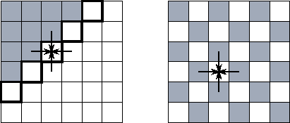
Figure 2.5:
Two finite difference update strategies, here applied on a two-dimensional
grid with a five-point stencil. In both figures, shaded grid points have already
been updated to step t+1 ; unshaded grid points are still at step
t . The arrows show data dependencies for one of the latter points. The
figure on the left illustrates a simple Gauss-Seidel scheme and highlights the
five grid points that can be updated at a particular point in time. In this
scheme, the update proceeds in a wavefront from the top left corner to the
bottom right. On the right, we show a red-black update scheme. Here, all the
grid points at step t can be updated concurrently.
This example indicates the important role that choice of solution strategy can play in determining the performance of a parallel program. While the simple Gauss-Seidel update strategy of Equation 2.2 may be appropriate in a sequential program, it is not ideal on a parallel computer. The Jacobi update strategy is efficient on a parallel computer but is inferior numerically. The red-black scheme combines the advantages of both approaches.
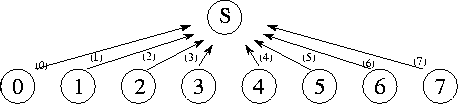
Figure 2.6: A
centralized summation algorithm that uses a central manager task (S) to sum
N numbers distributed among N tasks. Here, N=8 , and
each of the 8 channels is labeled with the number of the step in which they are
used.
A global communication operation is one in which many tasks must participate. When such operations are implemented, it may not be sufficient simply to identify individual producer/consumer pairs. Such an approach may result in too many communications or may restrict opportunities for concurrent execution. For example, consider the problem of performing a parallel reduction operation, that is, an operation that reduces N values distributed over N tasks using a commutative associative operator such as addition:

Let us assume that a single ``manager'' task requires the result S
of this operation. Taking a purely local view of communication, we recognize
that the manager requires values  ,
,  , etc., from tasks 0, 1, etc. Hence, we
could define a communication structure that allows each task to communicate its
value to the manager independently. The manager would then receive the values
and add them into an accumulator (Figure 2.6).
However, because the manager can receive and sum only one number at a time, this
approach takes
, etc., from tasks 0, 1, etc. Hence, we
could define a communication structure that allows each task to communicate its
value to the manager independently. The manager would then receive the values
and add them into an accumulator (Figure 2.6).
However, because the manager can receive and sum only one number at a time, this
approach takes  time to sum N numbers---not a
very good parallel algorithm!
time to sum N numbers---not a
very good parallel algorithm!
This example illustrates two general problems that can hinder efficient parallel execution in algorithms based on a purely local view of communication:
We first consider the problem of distributing the computation and communication associated with the summation. We can distribute the summation of the N numbers by making each task i , 0<i<N-1 , compute the sum:

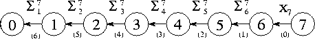
Figure 2.7: A
summation algorithm that connects N tasks in an array in order to sum
N numbers distributed among these tasks. Each channel is labeled with
the number of the step in which it is used and the value that is communicated on
it.
The communication requirements associated with this algorithm can be satisfied by connecting the N tasks in a one-dimensional array (Figure 2.7). Task N-1 sends its value to its neighbor in this array. Tasks 1 through N-2 each wait to receive a partial sum from their right-hand neighbor, add this to their local value, and send the result to their left-hand neighbor. Task 0 receives a partial sum and adds this to its local value to obtain the complete sum. This algorithm distributes the N-1 communications and additions, but permits concurrent execution only if multiple summation operations are to be performed. (The array of tasks can then be used as a pipeline, through which flow partial sums.) A single summation still takes N-1 steps.
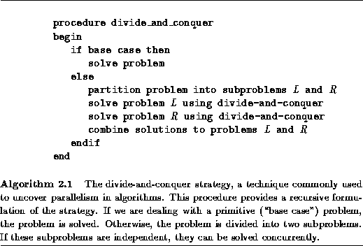
Opportunities for concurrent computation and communication can often be
uncovered by applying a problem-solving strategy called divide and
conquer. To solve a complex problem (such as summing N numbers),
we seek to partition it into two or more simpler problems of roughly equivalent
size (e.g., summing N/2 numbers). This process is applied recursively
to produce a set of subproblems that cannot be subdivided further (e.g., summing
two numbers). The strategy is summarized in Algorithm 2.1. The
divide-and-conquer technique is effective in parallel computing when the
subproblems generated by problem partitioning can be solved concurrently. For
example, in the summation problem, we can take advantage
of the following identity ( , n an integer):
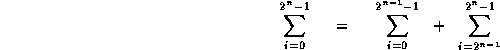
The two summations on the right hand side can be performed concurrently. They
can also be further decomposed if n>1 , to give the tree structure
illustrated in Figure 2.8.
Summations at the same level in this tree of height  can be performed
concurrently, so the complete summation can be achieved in
can be performed
concurrently, so the complete summation can be achieved in  rather than N
steps.
rather than N
steps.
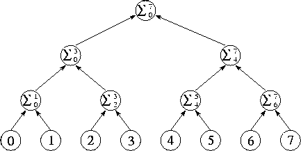
Figure 2.8:
Tree structure for divide-and-conquer summation algorithm with N=8
. The N numbers located in the tasks at the bottom of the diagram are
communicated to the tasks in the row immediately above; these each perform an
addition and then forward the result to the next level. The complete sum is
available at the root of the tree after  steps.
In summary, we observe that in developing an efficient parallel summation algorithm, we have distributed the N-1 communication and computation operations required to perform the summation and have modified the order in which these operations are performed so that they can proceed concurrently. The result is a regular communication structure in which each task communicates with a small set of neighbors.
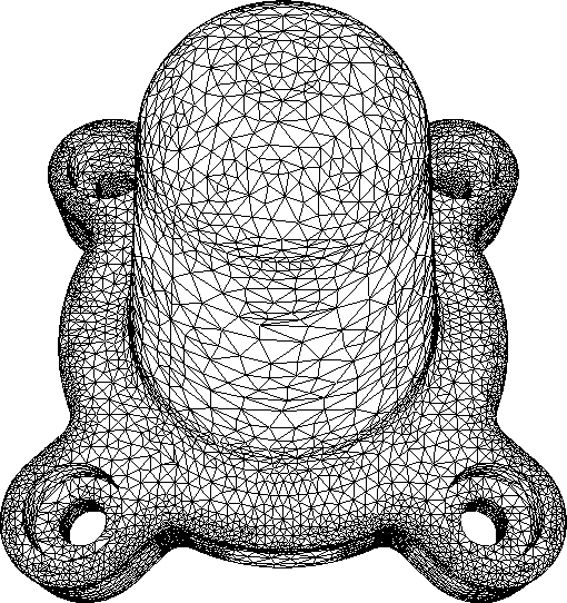
Figure 2.9:
Example of a problem requiring unstructured communication. In this finite
element mesh generated for an assembly part, each vertex is a grid point. An
edge connecting two vertices represents a data dependency that will require
communication if the vertices are located in different tasks. Notice that
different vertices have varying numbers of neighbors. (Image courtesy of M. S.
Shephard.)
The examples considered previously are all of static, structured communication, in which a task's communication partners form a regular pattern such as a tree or a grid and do not change over time. In other cases, communication patterns may be considerably more complex. For example, in finite element methods used in engineering calculations, the computational grid may be shaped to follow an irregular object or to provide high resolution in critical regions (Figure 2.9). Here, the channel structure representing the communication partners of each grid point is quite irregular and data-dependent and, furthermore, may change over time if the grid is refined as a simulation evolves.
Unstructured communication patterns do not generally cause conceptual difficulties in the early stages of a design. For example, it is straightforward to define a single task for each vertex in a finite element graph and to require communication for each edge. However, unstructured communication complicates the tasks of agglomeration and mapping. In particular, sophisticated algorithms can be required to determine an agglomeration strategy that both creates tasks of approximately equal size and minimizes communication requirements by creating the least number of intertask edges. Algorithms of this sort are discussed in Section 2.5.1. If communication requirements are dynamic, these algorithms must be applied frequently during program execution, and the cost of these algorithms must be weighed against their benefits.
The examples considered in the preceding section have all featured synchronous communication, in which both producers and consumers are aware when communication operations are required, and producers explicitly send data to consumers. In asynchronous communication, tasks that possess data (producers) are not able to determine when other tasks (consumers) may require data; hence, consumers must explicitly request data from producers.
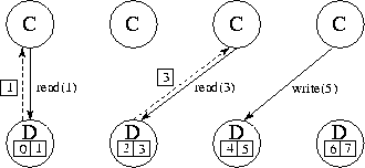
Figure 2.10:
Using separate ``data tasks'' to service read and write requests on a
distributed data structure. In this figure, four computation tasks (C) generate
read and write requests to eight data items distributed among four data tasks
(D). Solid lines represent requests; dashed lines represent replies. One compute
task and one data task could be placed on each of four processors so as to
distribute computation and data equitably.
This situation commonly occurs when a computation is structured as a set of tasks that must periodically read and/or write elements of a shared data structure. Let us assume that this data structure is too large or too frequently accessed to be encapsulated in a single task. Hence, a mechanism is needed that allows this data structure to be distributed while supporting asynchronous read and write operations on its components. Possible mechanisms include the following.
Each strategy has advantages and disadvantages; in addition, the performance characteristics of each approach vary from machine to machine. The first strategy can result in convoluted, nonmodular programs because of the need to intersperse polling operations throughout application code. In addition, polling can be an expensive operation on some computers, in which case we must trade off the cost of frequent polling against the benefit of rapid response to remote requests. The second strategy is more modular: responsibility for the shared data structure is encapsulated in a separate set of tasks. However, this strategy makes it hard to exploit locality because, strictly speaking, there are no local data: all read and write operations require communication. Also, switching between the computation and data tasks can be expensive on some machines.
Having devised a partition and a communication structure for our parallel algorithm, we now evaluate our design using the following design checklist. As in Section 2.2.3, these are guidelines intended to identify nonscalable features, rather than hard and fast rules. However, we should be aware of when a design violates them and why.
© Copyright 1995 by Ian Foster